There is a block diagram that turns up in every satellite dynamics course. A summing junction on the left takes Earth's gravity, third-body pull from the sun and moon, the nonspherical corrections, atmospheric drag, solar pressure and rocket thrust. Everything adds into one acceleration vector, that vector goes through two integrators, out comes position, and position feeds back around to compute gravity again.
That is Cowell's method. It is what the equation of motion literally says, and it is what almost everyone builds first. (The version that prompted this post is Dr. Andrew Motes', and it is a clean statement of the form.)
The other classical answer is Encke's method, and the first thing to say about the pair is the thing most often got wrong: they are the same physics. Both solve Newton's equations. Neither is "more Keplerian" than the other. The difference is entirely numerical — it is about what you hand to the integrator, and therefore about which error you end up paying for.
I care about the distinction because it sits in the middle of galaxy, the n-body space simulation I have been building — a persistent world where ships and stations orbit real bodies and the physics has to stay honest for months of continuous simulated time rather than for the length of a mission study. That turns the textbook trade into an engineering one: which error can you live with, integrated over a system that never stops. It also turned out to be a better example than I wanted, and I will come back to it at the end.
Everything below is measured on a real perturbed two-body problem rather than asserted. The figures come out of an integration you can re-run, and where the numbers disagreed with what I had written, I changed what I had written.
Cowell: integrate everything
Write down every acceleration acting on the spacecraft, add them, integrate twice.
What it is good at is generality, and the generality is not a small thing.
There is no reference orbit to maintain, so there is nothing to rectify, nothing to re-osculate, and no bookkeeping about when the reference has gone stale. A new force model — a better atmosphere, radiation pressure, a thrust profile — drops into the sum without touching anything else. And crucially, nothing special happens when the dominant body changes. A probe leaving Earth for Mars is handled by the same equation throughout: the Earth term shrinks, the Mars term grows, and at no point does the software need to notice. That property is why Cowell is the workhorse for interplanetary trajectory work, and it is the strongest argument in its favor.
What it costs is that your error budget is set by the biggest term in the sum.
In low Earth orbit the central −μ/r³ term dwarfs the oblateness correction — measured at 867× on the orbit used for the figures below, which is 2.9 orders of magnitude, and I had written "three to four" before running it. Drag and solar pressure are smaller again. All of it goes through the same two integrators. So the truncation error is dominated by the central-body force — which happens to be the one term with an exact closed-form solution. You are asking a numerical integrator to rediscover Kepler, imperfectly, on every single step, and the interesting physics then has to share whatever error budget is left over. In practice that means small steps and a lot of them.
Encke: integrate only the difference
Encke's answer is to subtract the part you already know. Pick an osculating two-body reference orbit — the trajectory the spacecraft would follow with no perturbations — propagate it analytically, and numerically integrate only the deviation.
The large central-body term leaves the integrator entirely and is carried in closed form. What remains going through the numerics is small, so the error scales with the perturbation rather than with the whole orbit. For a satellite in a well-behaved orbit where perturbations are a thousandth of the central force, that buys a large factor in accuracy at the same step size.
It buys much less in step size, and I had this wrong too. I first wrote "an order of magnitude or more in step size." At fourth order, the 15× accuracy factor measured below is a 1.97× step-size factor — the fourth root. An order of magnitude in step would need 10⁴ in accuracy.
What it costs is machinery, and three specific problems.
Rectification. The deviation grows. As it does, the formulation loses the very property that justified it — eventually δ is no longer small and the advantage evaporates. So you must periodically stop, re-osculate a fresh reference orbit from the current state, and reset δ to zero. That means a criterion for when to rectify, a decision about what triggers it, and a discontinuity in the bookkeeping every time it fires.
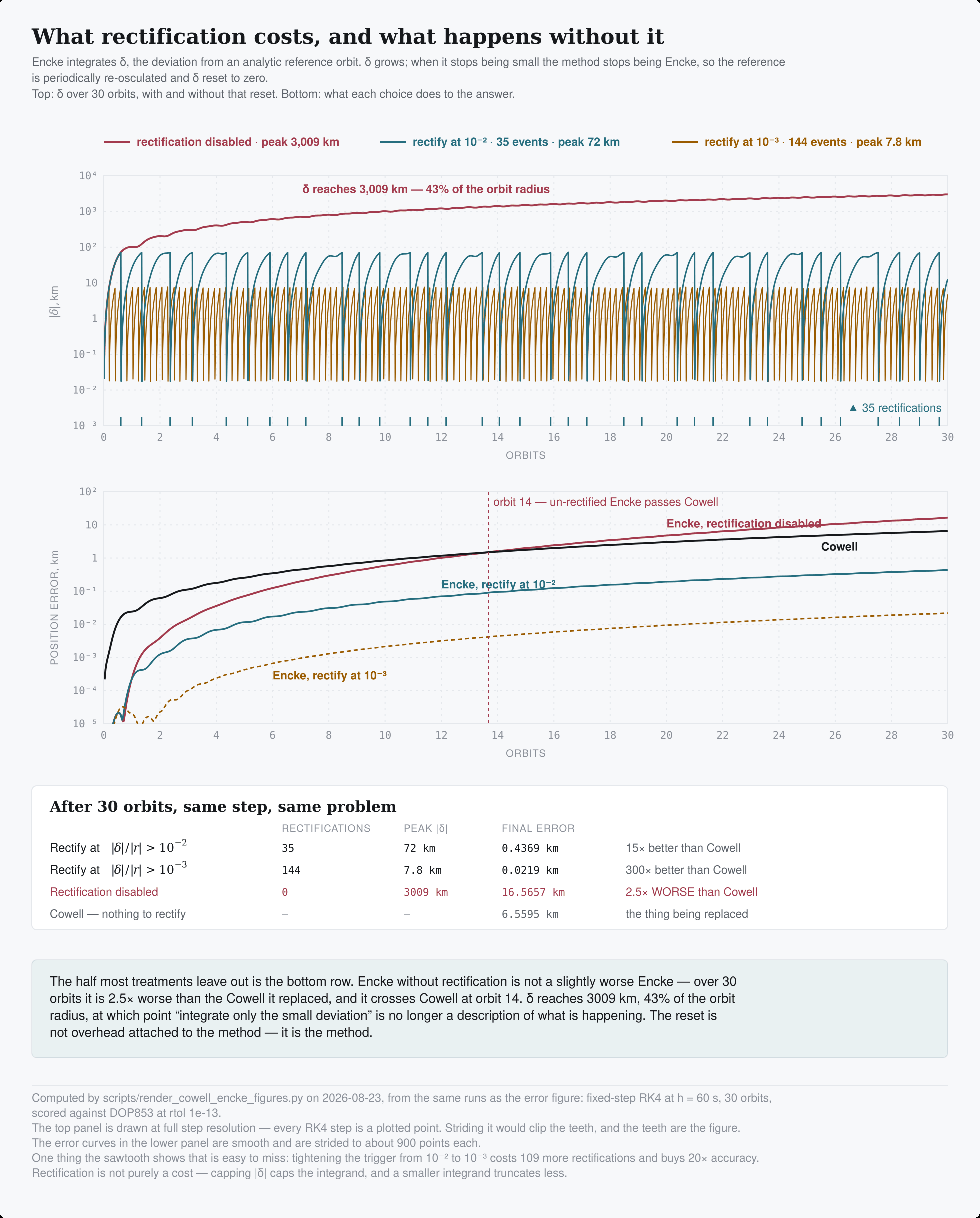
Rectification is not purely a cost, which surprised me. Capping |δ| caps the integrand, so resetting more often also cuts truncation error: tightening the trigger from 10⁻² to 10⁻³ costs 109 more rectification events and buys 20× the accuracy. How often to rectify is an accuracy knob, not just overhead. And turning it off is not an option — with rectification disabled, |δ| reaches 3,009 km, 43% of the orbit radius, and the error crosses above plain Cowell at orbit 14 and finishes 2.5× worse. An Encke without rectification is worse than the Cowell it replaced.
A changing dominant body. Encke needs to know what it is perturbing from. When the spacecraft passes from one body's influence to another's, the reference has to change too — and that is precisely the transition Cowell handles by doing nothing at all. Encke is awkward exactly where Cowell is graceful.
Catastrophic cancellation, which is the one that bites in practice. Computing the perturbation from a third body means differencing two nearly-equal accelerations — one on the spacecraft, one on the reference body. Both are large; their difference is small; and in floating point the subtraction destroys most of the significant digits. A naive Encke implementation can be less accurate than the Cowell it replaced, for this reason alone.
The standard fix is Battin's f(q) formulation, which computes that difference in closed form rather than by subtraction:
It is not glamorous and it is the difference between a working Encke and a broken one. If you find yourself implementing Encke and you have not thought about cancellation, you have not implemented Encke.
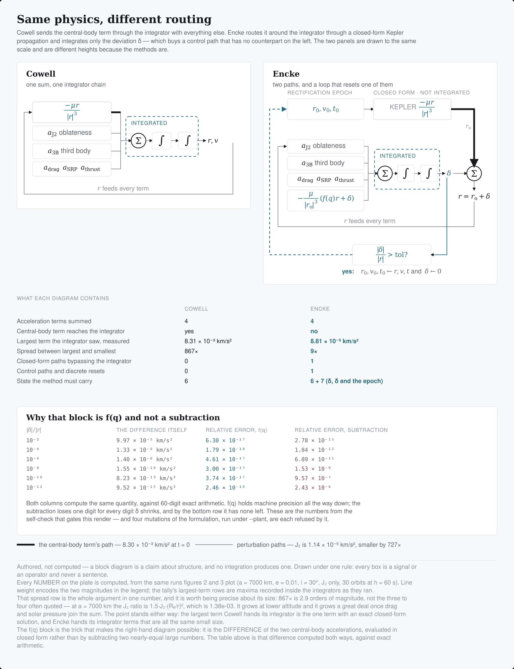
The structural difference in one picture. Cowell feeds the central term into the same integrator as everything else. Encke splits it off into a closed-form propagation and hands the integrator only what is left.
Which one, when
The honest rule is a ratio: how large are the perturbations relative to the central term, and how long does the reference stay good?
Encke earns its complexity on long arcs around a single dominant body with small perturbations — the classic Earth-satellite case, where the central force is overwhelming and stays that way for thousands of orbits.
And the Earth satellite is not the best case. Natural satellites are. The orbit measured above runs a perturbation ratio of about 1.2 × 10⁻³. Callisto around Jupiter sits at 4.2 × 10⁻⁴ — that is Ganymede at closest approach, with the solar tide another order below at 3 × 10⁻⁵. Phobos around Mars sits at 3.9 × 10⁻⁴, dominated by Mars' oblateness. Both are roughly three times deeper into Encke's territory than the case these figures use, and Phobos completes 1,145 orbits a year, so the long-arc condition is met about as emphatically as it can be.
That is the shape to look for: a primary that overwhelms everything, a perturbation that is genuinely a rounding error against it, and enough revolutions that a small per-step advantage compounds into a large one. A moon is a better Encke problem than a spacecraft, because nobody ever fires its engine.
Cowell earns its simplicity when perturbations are comparable to the central term, when the dominant body changes, when the force model is unusual or changing, or when engineering simplicity is worth more than steps per second.
And on this problem, at equal wall clock, Cowell wins outright. Encke's right-hand side costs about 5× Cowell's, because every step pays for a Kepler solve. Run Cowell at half the step size and it costs less wall time than Encke at the full step and comes out about twice as accurate. Break-even needs a force evaluation expensive enough to swamp the Kepler solve — roughly 12 µs, about 4× this J2-only model. A 70×70 geopotential clears that comfortably; J2 alone does not.
That number is implementation-dependent in a way the accuracy results are not — a pure-Python Kepler solve against a trivial force model is about as unfavorable to Encke as it gets, and the figure says so. But the direction is the point: Encke's advantage was formulated when arithmetic was scarce, and it is less scarce now. A method with no reference to maintain and no rectification criterion to tune has real value that never shows up in a truncation-error analysis.
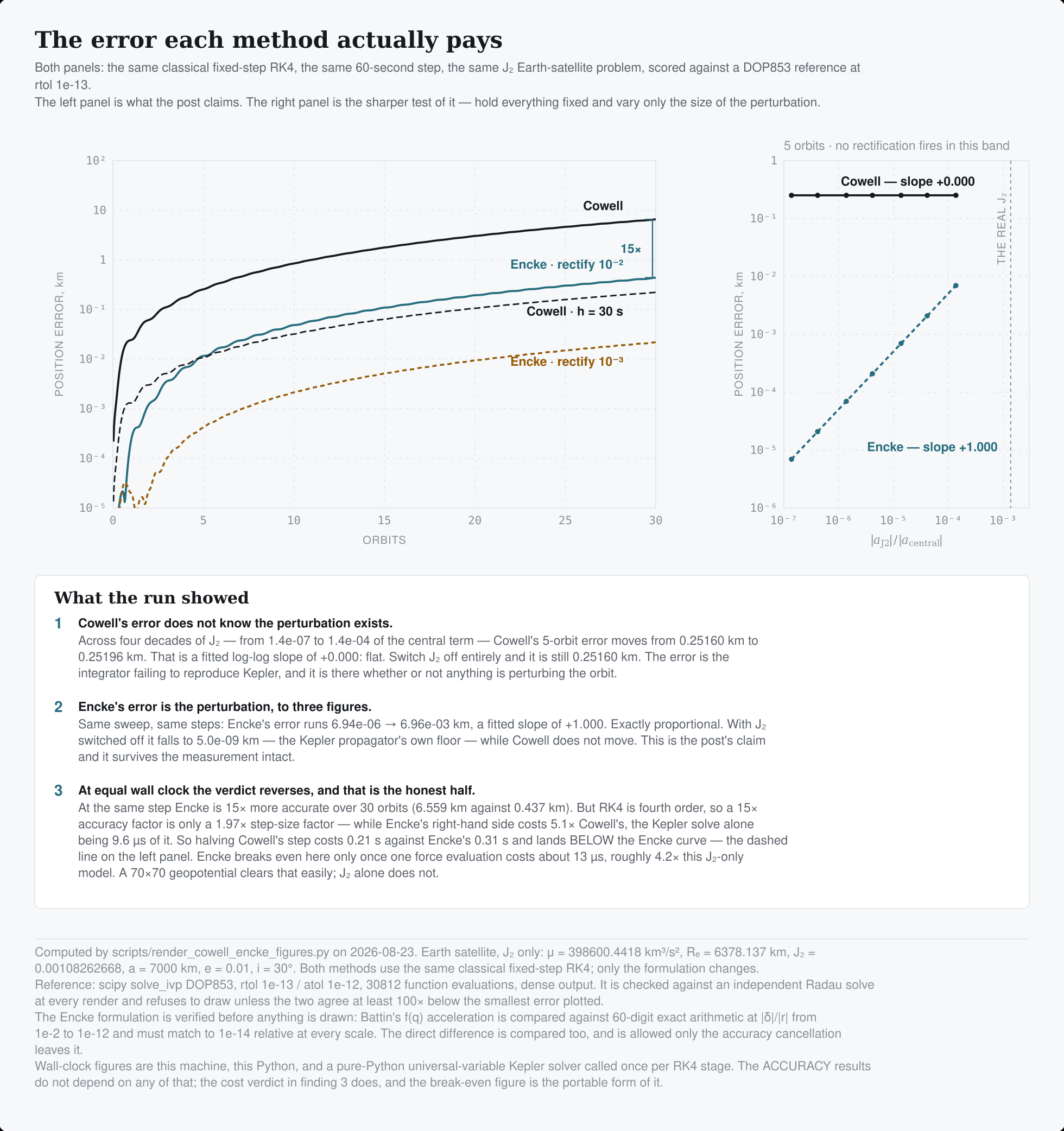
Both curves come from the same problem integrated at the same step size, scored against a high-accuracy reference. Nothing here is drawn; where the run disagreed with what I had written, I changed what I had written.
The sharpest result is not the gap, it is the slope. Hold everything fixed and scale J2 across four decades: Encke's error tracks it with a fitted log-log slope of +1.000 — exactly proportional to the perturbation, which is the whole claim. Cowell's slope is +0.000. Its error does not care how large the perturbation is, because its error is not about the perturbation. Switch J2 off entirely and Cowell is still wrong by the same amount — that residue is the integrator failing to reproduce Kepler, and it is there whether anything perturbs the orbit or not. Encke with J2 off falls to the Kepler propagator's floor.
That is a stronger statement than the one I set out to make, and it only exists because the figure was computed rather than drawn.
There is also a decision hiding underneath both, which is the choice of integrator. A symplectic method like velocity Verlet bounds energy error but says nothing about phase — a body can be on exactly the right orbit and in the wrong place along it. That failure mode is independent of the Cowell/Encke choice, and it is easy to mistake one problem for the other.
A live example: the name is not the method
I have been working on an n-body space simulation whose physics core contains a function called encke_substep_loop. Its architecture specification describes it as Encke's method, and that specification is genuinely careful — its terminology section defines the distinction better than most textbook treatments:
The benefit of Encke is not "no leapfrog" — it is "leapfrog only the small perturbation, get the large central-body force exactly via Kepler".
The kernel does something else. Its delta_r is a plain frame subtraction — the ship's state relative to the reference body — and it then computes the full −μ/r³ numerically and integrates that, every substep. There is no analytic Kepler reference anywhere in the loop, and therefore nothing to rectify. It is Cowell in a body-centered frame, with Battin's f(q) correctly applied to the third-body term — the Encke idea surviving in the one place cancellation was actually eating the answer, but not in the main integration.
The part I find genuinely interesting is that the same specification, two paragraphs earlier, defines the alternative and warns about it:
Raw leapfrog = Velocity Verlet of the full ship state (no Kepler reference). Acceptable for body-on-body N-body where the central force is diffuse, problematic for ship-around-body where the central force dominates.
The ship path is ship-around-body with a dominant central force. The document may be warning about its own implementation, and it cannot tell you so, because it does not believe the two are the same thing.
There is a further turn to it. The same simulation carries a separate correction for its bodies — a phase-only nudge that decomposes each moon into osculating elements, compares its mean anomaly against a frozen Kepler clock, and pulls it back. It exists because a symplectic integrator bounds energy error and says nothing about phase, and the drift that motivated it was measured on Callisto: 78,375 km along-track, walking millions of kilometers off true orbit if left alone.
That correction is already using a Keplerian reference. It just applies it as a post-hoc nudge rather than as the thing being integrated — which is Encke's idea arriving through the back door, to patch a symptom that Encke's formulation addresses at the root. And Callisto, as it happens, is one of the most favorable Encke problems in the solar system.
I should say that I got this wrong myself. I read the function name and the spec, wrote a post on that basis, and had to retract it after reading the arithmetic. The name was load-bearing in my reasoning and it should not have been.
What to take from it
Choose by which error you can afford, not by which method sounds more sophisticated. Cowell's cost is that the integrator spends its precision on a term you could have written down. Encke's cost is a reference to maintain, a rectification criterion to tune, and a cancellation problem that will silently eat your accuracy if you do not handle it. Both are defensible; they are defensible in different situations.
And a smaller lesson that generalizes well past orbital mechanics: a claim about accuracy is a claim, and it should be checked against the arithmetic rather than against the identifier. "The central force is exact" is the sentence that would justify a step-size budget and every tolerance built on it. It is worth about thirty seconds to confirm that the code agrees.